在USYD上NLP课程的时候对于w2v一直十分的困惑，只知道其输入输出的区别以及目的，没有深究其原理以及实现方式。今天对于其中两个模块进行详细的研究，算是补齐了之前的一小块拼图。其中的两个优化方法都是对于复杂度的降低，一个是对于词表的降低，另一个是对于损失函数计算方法的降低。是通过近似和模拟的方式去考虑以实现降低的计算。写篇文章记录一下，下次忘记了有地方找（bushi （：

Word2vec

If the encoding use the one hot encoding to represent the word. The dimension will be huge, and the matrix will be sparse. Even the PCA could be applied.

Also, this way could have another limitation, that is the semantic could not be represent well. For instance, the value of COS in similar wards are 0, they show the totally different.

Thus, the word2vec come up. Its not a model, but a tool.

It concludes CBOW and Skip-gram

First, define the size of window, if the window is 2, that will be [t-2,t-1,t,t+1,t+2]

For Skip-gram, the t is used to predict the context, i.e., 2 backward and forward.

For CBOW, the context is used to predict the word in the middle.

In terms of the input of CBOW, that is the 4 words, calculate the average values, and pass into the function of softmax to get the result.

Skip-gram is similar, remove the operation of average, due to it is itself, no matter need the average.

In the word2vec, there are 2 optimised method, negative sampling and hierarchical softmax.

negative sampling means “ABCDE” - middle word is C, context is AB and DE. postive sample is CA, CB, CD, CE, which is the concurrence of word in sentence. However, it need go through the whole dictionary, waste too much resource. So, create the negative samples CC,CF, etc. It also only choose K sample randomly for the simplicity.

Hierarchical softmax: first create the tree with order, 霍夫曼树, the final possibility is the value times among the path that searching in the tree. binary classification for each path, get the possibility, then multiply it. It means to reduce the computational resources, comparing to the go through whole data. The operation is the similar value, not exactly accurate.

Also, there is another concept called subsampling, the possibility decided by the frequent, aiming to remove the high frequent word, like ‘the’, which no include much meaning in the word.

Comparison: CBOW train faster than Skip-gram, but Skip-gram could get better vector representation.

CBOW only predict one word, but the skip-gram predict 2K times, K means the window size. So, skip-gram will get better vector representation for low-frequent, due to its training repeat more times.

XLNET

Original address of paper

https://arxiv.org/abs/1906.08237

Reason the idea come up

XLNET uses the AR method to implement the language model.

AR has the unidirectional limitation. And, AE has issue in MASK. In fine tuning phase, input of BERT without data with MASK, showing the discrepancy, and author thought that BERT assume the predicted token as independent word is oversimplified the natural language. Therefore, the XLNET is created to leverage best of AR and AE to avoid the limitation.

Main idea of the technology

Firstly, standing at the conventional AG mode

permutation

instead of forward or backward of sequence, XLNET have all possible permutations

this operation aims to get the bidirectional context like BERT.

In detail, XLNET create the all permutations and randomly choose some cases to predict some masked words in end of sequence. e.g., 1,2,3,4,5,6,7 → use 1,2,4,5,6,7 to predict 3. No matter the order is.

Meanwhile, how to decide the length of predict token? there is a hyper parameter K, which is equal the length of sequence dividing by length of predicted token.

The implementation of permutation is the mask in transformer’s attention.

Two-Stream Self-Attention

In the case of 1342 and 1324, when we want to predict the place of 3, i.e. (target 4 or 2), the word they could see are same, which is not right. Therefore, we introduce the Two-Stream Self-Attention.

1. h, the content representation
2. g, the query representation, access to contextual and position information, but without content

Thinking

The paper also incorporating the idea from Transformer-XL. (seems aims for long text task) (relative position encoding and fragment loop?)

The details of Transformer XL is not clear for me, maybe after learning for it and get deeper understanding for XLNET

Terms appear in the paper

AR: Autoregressive Language model

using the sequential direction to predict the next word, that is the single direction, e.g. GPT2

AE: Autoencoding Language model

utilise the context. i.e., BERT. It includes the MLM (masked language model) and NSP (next sentence prediction). NSP is to deduce the inference relation, MLM replace some word with MASK, and to predict the position with MASK.

tBERT

Original address of paper

https://www.aclweb.org/anthology/2020.acl-main.630.pdf

Reason the idea come up

The semantic similarity could provide additional signal and information to model. Also, the integration of the domain could effectively help the model get better performance. That is the reason tBERT come up.

Main idea of the technology

First create the place for CLS in BERT, representing the domain of the input.

The input of sentences put into the topic model and get the average value.

At the meantime, the input the sentences into the BERT

The paper not mention the detail design of loss, from my understanding, the CLS should be included in the loss, and no other digest article for the tBERT, may it should be confirmed for the further research.

Thinking

Fine tuning could also helps model to deal with the domain shift, but the experiment showed that the result of tBERT is better than the fine tuning, especially for the specific domain, e.g., medical, finance, etc.

UniLM

The term stands for Unified Language Model Pre-training for Natural Language Understanding and Generation

Original address of paper

https://arxiv.org/pdf/1905.03197.pdf

Reason the idea come up

The reason of the BERT not good for NLG is the MLM(mask language model), which is not the same with the target of generation task. Except the masked position, other words are seen for model. Therefore, to improve the NLG performance of BERT, one way to handle is get better NLG ability.

Main idea of the technology

The author thought that the natural way to control the model is the mode of information input in the model. E.g., the access to the context of the word token to be predicted. The paper proposed the 3 ways: bidirectional LM, unidirectional LM, sequence-to-sequence LM.

For the special token, SOS, EOS stand for start and end of sentence. They helps to improve the ability of NLU and NLG, it marks the end of sequence, and help model to learn the when to terminate the NLG task.

In the unidirectional LM, comprised by left to right and right to left LM. Taking the example of left to right, the x1, x2, [mask], x4. The representation of mask only x1 and x2

In the bidirectional LM contains both directions context to represent the masked token.

In the sequence to sequence LM, the input has segment, that is the source and the target segments. SOS, t1 ,t2, EOS t3, t4, t5, EOS. t2 could access the first 4 tokens, t5, could only get the first 6 tokens. (including the SOS and EOS)

Also, the paper mentioned that the 1/3 time use the bidirectional LM objective, 1/3 time used the seq2seqLM objective, and the left to right and right to left are 1/6 of the time be set as the objective. By this strategy, the final objective of UniLM could be achieve, i.e., generative performance.

In more details, the initialisation of UniLM used BERT-large, and the strategy of mask is same with BERT, but 20% of chance will be bigram or trigram, to improve the predictive performance.

Terms appear in the paper

There are two new terms of NLP:

NLU: Natural language understanding

NLG: Natural language Generation

The concepts are not brand new, but the abbreviations are good for extension

RoBERTa

Original address of paper

https://arxiv.org/abs/1907.11692

https://zhuanlan.zhihu.com/p/149249619

根据知乎的文章，总结出以下几点特征：

1. 用更长的时间和更大的BS，训练更多的数据
2. 去掉BERT中的NSP（next sentence prediction)
3. 在更长的句子上训练
4. 根据训练数据动态的改变mask模式

Reason the idea come up

从BERT的角度来说，masking是在预处理的时候执行Masked Language Model. In random masking, BERT will select the 15% word in each sentence, and with 80% chance replaced by MASK, 10% chance replaced by other random word, 10% keep the same. Recall the COMP 5046 unit, assignment, there are same. Thus, the model target is to predict the place be marked.

Also, BERT could predict the adjacent position relationship between sentences, that is called Next Sentence Prediction(NSP)

Difference:

其中比较大的变化是对于mask的处理方式不同

BERT是在pre-precessing的时候对于masking进行处理，这样一来masking是静态的，也就是对于每一个epoch来说masking的结果是一致的。为了避免这样的情况，会对数据进行复制，作出不同的静态masking进行训练。但还是会出现重复的现象。

而RoBERTa使用动态masking，在序列进入模型之前才处理masking的任务。

RoBERT remove the task of NSP, it consider this task is not improve the performance in expected.

思考：BERT输出信息的继续挖掘以达到更好的语义理解

On the sentence embeddings from pre-trained language models

this is the address for original paper

https://arxiv.org/pdf/2011.05864.pdf

The problems proposed in the paper mainly discuss the:

1. why low performance of text matching in BERT for unsupervised task. Is that lacking of the sentiment information or wrong way to digging these information?
2. If lacking of digging, how to utilize them.

论文给出的结论是我们对于BERT的输出信息利用不够强

论文中提出了一个方式，去映射BERT sentence embedding, called BERT-flow.

其启发是来自于1. 高频的偏差，对于高频词语的space来说，可能会导致向量的偏移，这会导致对于向量之间关系不按照我们所想的方式进行发展。2.sparse word会在BERT空间中比较稀疏（低频词），以及产生一些洞。这些洞会导致语义理解的难度

基于这两个问题， paper提出了一个转换的方式：

BERT embedding space to standard Gaussian latent space

从而实现了基于流的标定来帮助建立更加正确的BERT词向量

FastBERT

https://aclanthology.org/2020.acl-main.537/

首先给出模型的提出原文地址

https://zhuanlan.zhihu.com/p/127869267

对于FastBERT的定义和解读，知乎这篇文章讲的十分优秀，可以仔细阅读

简单来理解，单纯使用BERT对样本进行预测工作需要经过完整的网络，FastBERT的主要目的是为了让降低计算。

1. 从蒸馏的角度来说是创建一个全新的学生网络去拟合本地的大BERT模型从而实现对模型的简化。
2. 但是FastBERT的思想是对于模型进行改造。聚焦于一些简单的样本，也就是不需要通过整个网络就可以进行分类的样本进行优化。解决方案为：给每一层后接上分类器。这样主要的结构就出现了。

作者称之BERT模型为主干，Backbone

每一个分类器为分支，Branch

这一过程作者称之为自蒸馏，在pre-train & fine-tuning 的时候只更新主干，tuning结束之后freeze主干用branch获得蒸馏结果

总结，fastBERT主要思想是提前输出简单样本，来减少模型的计算压力，从而提高推理速度。优点：不需要改变主要的BERT结构（相比于Distill-BERT）

思考：如何去决定当前批数据经过的层数，如何去定义？

在原文中提到，不确定性高于speed的将会被传入下一层，低于speed的就停止传递

其中，对于不确定性的定义是当前批的数据的煽值（正则化），其中包括一些假设：低不确定性对应高精度。这样子理解，speed在原文中的意义就是threshold，去定义以及划分不确定性的高低。越高的speed，越高的层收到的样本就越少，也就意味着门槛变低，更多的样本被直接输出，从而提高了模型的计算速度。

至于模型的loss计算，GPT给出的解释为分类loss和层选择的loss（CE, MSE[选择的层和全部的层]）但是觉得与原文有些出入，还需要进一步研究。（对于损失函数的观点未经证实）

本文记录了阅读FastBERT paper的笔记以及对于前辈的知识总结进行归纳。大致了解了FastBERT的思路和实现原理，但对于原文中的KL散度分布还有些困惑，需要进一步研究。

Knowledge Distillation

Original address of paper

https://zhuanlan.zhihu.com/p/75031938

The main idea of the knowledge distillation is “forget the models in the ensemble and the way they are parameterised and focus on the function”

Main idea of the technology

https://arxiv.org/abs/1503.02531

在Hinton原文中指出训练时就如同毛毛虫吃树叶来积攒能量，在使用神经网络的时候既做了吃树叶又繁殖的任务，导致效率低下。因此对于这样的问题，希望将一个复杂的模型转变到简单的模型，也就是知识蒸馏做的事情。

蒸馏的过程就是将训练的大模型的内容总结到小模型中，已达到模型复杂度和精度的平衡。在这里会有两个模型，较大的为老师模型，小的模型为学生模型，老师模型通过对于hard targert 进行训练，而学生模型通过老师模型的输出进行收敛。

To achieve training of the student network, the paper mentioned that adding a temperature to scale down the target before input into the softmax. (i.e., exp(zi/T) / sum(exp(zi/T))) The more larger T in formula, the more smooth distribution the result will be.

The loss function is a * soft + (1-a) * hard, i.e. the trade-off between them.

in general, the larger soft distribution will get better performance in test.

1. 训练大模型，也就是使用hard taget， 也就是不对标签做处理
2. 通过老师模型计算soft target
3. 训练小模型
   1. 设置相同T计算结果与soft target 计算loss （from 2）
   2. 设置T为1，也就是hard target计算loss
4. 学生模型T设置为1作为最后的预测

Summary

The reason knowledge distillation worked is the too sharp distribution of result makes loss function not effect the model, i.e., except the true label, outputs are too close to 0, making the model could not learning anymore. Thus, the introducing of the T to scaling down the result helps to get smooth distribution. In this way, get simper model and better convergence of model.

SpaCy

Quick Start

1. It contains the pip installation in python
2. created a english based nlp object
3. input some text to create the object of document
4. operations demo that can get the text from token
5. span of the token in text

1
2
3
4
5
6
7
8
9
10
11
12
13
14
15
16
17
18
19
20
21
22
23
24
25
26
27

# 1. installation
!pip install spacy

# 2. Create a blank English nlp object
nlp = spacy.blank("en")

# 3. Created by processing a string of text with the nlp object
doc = nlp("Hello world!")

# 4. Index into the Doc to get a single Token
token = doc[1]

# Get the token text via the .text attribute
print(token.text)

# Iterate over tokens in a Doc
for token in doc:
    print(token.text)

# 5. Create another document with text
doc = nlp("Hello NLP class!")

# A slice from the Doc is a Span object
span = doc[1:3]

# Get the span text via the .text attribute
print(span.text)

demonstrations of is_alpha, is_punct, like_num

1
2
3
4
5
6
7
8
9
10
11
12
13
14

doc = nlp("It costs $5.")
print("Index:   ", [token.i for token in doc])
print("Text:    ", [token.text for token in doc])

print("is_alpha:", [token.is_alpha for token in doc])
print("is_punct:", [token.is_punct for token in doc])
print("like_num:", [token.like_num for token in doc])

# output:
# Index:    [0, 1, 2, 3, 4]
# Text:     ['It', 'costs', '$', '5', '.']
# is_alpha: [True, True, False, False, False]
# is_punct: [False, False, False, False, True]
# like_num: [False, False, False, True, False]

Part of Speech

Load the small english pipeline to achieve the pos

1
2
3
4
5
6
7
8
9
10
11
12
13
14
15
16
17
18
19
20
21
22
23
24
25
26
27

!python -m spacy download en_core_web_sm

# Load the small English pipeline
nlp = spacy.load("en_core_web_sm")

# Process a text
doc = nlp("She ate the pizza")

# Iterate over the tokens
for token in doc:
    # Print the text and the predicted part-of-speech tag
    print(token.text, token.pos_, token.pos)

# result: 
# She PRON 95
# ate VERB 100
# the DET 90
# pizza NOUN 92

# also the token.head returns the syntactic head token
for token in doc:
    print(token.text, token.pos_, token.dep_, token.head)
    
# She PRON nsubj ate
# ate VERB ROOT ate
# the DET det pizza
# pizza NOUN dobj ate

Name Entity Recognition

1
2
3
4
5
6
7

# Process a text
doc = nlp("Apple is looking at buying U.K. startup for $1 billion")

# Iterate over the predicted entities
for ent in doc.ents:
    # Print the entity text and its label
    print(ent.text, ent.label_)

Matching

1
2
3
4
5
6
7
8
9
10
11
12
13
14
15
16
17
18
19
20
21
22
23
24
25
26
27

# Import the Matcher
from spacy.matcher import Matcher

# Load a pipeline and create the nlp object
nlp = spacy.load("en_core_web_sm")

# Initialize the matcher with the shared vocab
matcher = Matcher(nlp.vocab)

# Add the pattern to the matcher
pattern = [{"TEXT": "iPhone"}, {"TEXT": "X"}]
matcher.add("IPHONE_PATTERN", [pattern])

# Process some text
doc = nlp("iPhone X news! Upcoming iPhone X release date leaked")

# Call the matcher on the doc
matches = matcher(doc)

# Iterate over the matches
for pattern_id, start, end in matches:
    # Get the matched span
    matched_span = doc[start:end]
    print('"{}" - match for pattern {} in span ({}, {})'.format(matched_span.text, pattern_id, start, end))
    
# "iPhone X" - match for pattern 9528407286733565721 in span (0, 2)
# "iPhone X" - match for pattern 9528407286733565721 in span (5, 7)

in match pattern, LEMMA contains the multiple variations of the word

1
2
3
4
5
6
7
8
9
10
11
12
13
14
15
16

pattern = [
    {"LEMMA": "love", "POS": "VERB"},
    {"POS": "NOUN"}
]
matcher = Matcher(nlp.vocab)
matcher.add("LOVE_PATTERN", [pattern])

doc = nlp("I loved vanilla but now I love chocolate more.")

matches = matcher(doc)
for pattern_id, start, end in matches:
    matched_span = doc[start:end]
    print('"{}" - match for pattern {} in span ({}, {})'.format(matched_span.text, pattern_id, start, end))

# "loved vanilla" - match for pattern 4358456325055851256 in span (1, 3)
# "love chocolate" - match for pattern 4358456325055851256 in span (6, 8)

1
2
3
4
5
6

Operators and quantifiers let you define how often a token should be matched. They can be added using the "OP" key. "OP" can have one of four values:

- An "!" negates the token, so it's matched 0 times.
- A "?" makes the token optional, and matches it 0 or 1 times.
- A "+" matches a token 1 or more times.
- And finally, an "*" matches 0 or more times.

Word Vector

SpaCy contains the word vector in medium pipeline

It could output the word vectors and calculate the similarity of tokens

1
2
3
4
5
6
7
8
9
10
11
12
13
14
15
16
17

# Load a larger pipeline with vectors
nlp = spacy.load("en_core_web_md")

# Look at one word vector
doc = nlp("I love chocolate")
print(doc[2].vector)

# Compare two documents
doc1 = nlp("I like fast food")
doc2 = nlp("I like pizza")
print("Comparing sentences:", doc1.similarity(doc2))

# Compare two tokens
doc = nlp("I like pizza and pasta")
token1 = doc[2]
token2 = doc[4]
print("Comparing 'pizza' and 'paste':", token1.similarity(token2))

Reference

1. https://course.spacy.io/en/
2. https://spacy.io/

Lecture 1

N-Gram LMs

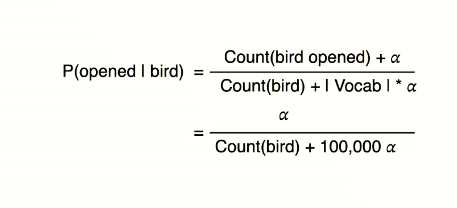
The 4 ways to deal with the unseen word sequence

smoothing:

discounting:

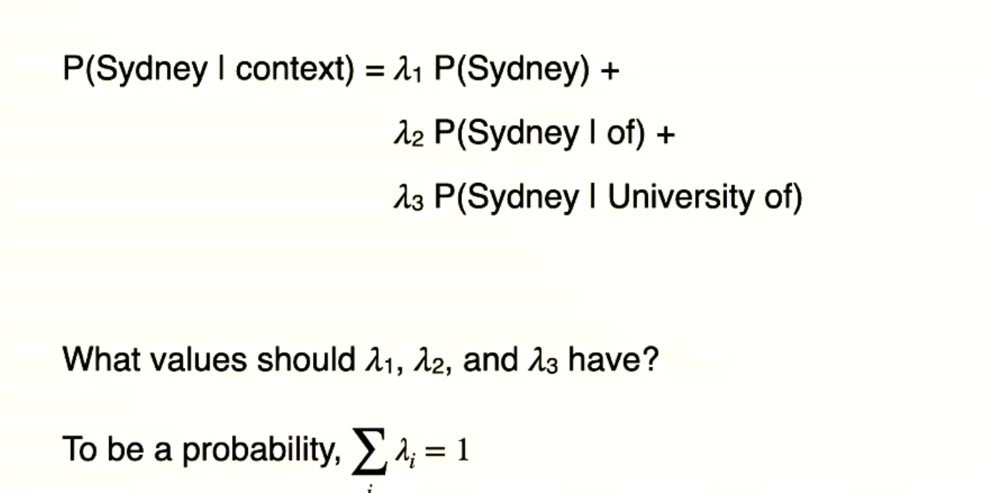
Interpolation: using the multiple N-Gram probability

Kneser-Ney smoothing:

Lecture2

Lecture3

Lecture4

Note the formula macro and micro F1 score — ass2

Not the find_best_socre initial number should be negative — ass2

directly using average will make some features vanish (+ and -), also the order is meaningless

in slide, NER page 66

labels number * length * length means:

each token in sequence is possible for start or end, that is length * length

then, each span can be predicted as each label

so, the output should be (labels * length * length)

Lecture 5

beam search

in nature, greedy search is to find the local optimal solution in each step

Lecture 6

the label in current word from LSTM purely, B I O possibility(sum as 1)

score = current label p * best (previous p * transfer p)

it from

score = current label p * best (i.e. DP * transfer model)

DP refers to the optimal route in choice

transfer model refers to the Markov model

co reference

dependency parsing

Lecture 7

Lecture 8

disadvantages of self-attention

problem:

non-linear lacking

order lacking

resolve:

feedforward layer

additional position vector

issue: the length of the position vector is fixed, not flexible enough
the mask is for ignoring the future word in the training process, it lets the model know what is known in this step, and what is the prediction in this step. In math, put the infinite negative value for future words and dot the product in the current word
the multiple layers of self-attention are used to build better representation of the word

query: curve line

key: embedding word

value: passing into the weighted value

Lecture 10

data can from

fineweb

common craw

Lecture 11

Review

The content below is the missing slide week.

parsing, 句法分析, identity the grammar structure by sub-phrases

The span in the sentence called the phrase

treebanks

Method: Dependency Parsing / Grammar

compute every possible dependency to find the best score

Or, choose a way to get the best overall score

co-reference

COMP 5329

Lecture 2

P9 XOR

P31 Activation

P36 CE

P37 KL, Entropy

P38 SoftMax

p36, p37 two attributes cross-entropy loss issue?
the disadvantage of batch gradient descent is when N is too large, the computation is very expensive, but the one example SGD only uses the single example. It may not be the best, due to the random.

mini-batches SGD: divide into mini-batches, in each epoch calculate the gradient

extension content:

sensitivity? make the back propagation similar to the feedforward

Lecture 3 GD

Different gradient descent.

Challenges: proper lr, same lr, saddle point

P9-10 Momentum

P11 NAG

P17 Adagrad

P21 Adadelta

P25 RMSprop

P26, 27 Adam

P34 Initialization

Batch Gradient descent: Accuracy

Stochastic gradient descent: efficiency

Mini-batch gradient descent: trade-off of accuracy and efficiency

Momentum is to update SGD, to accelerate and dampen oscillation

increase the momentum term in the same direction, reduce in change direction

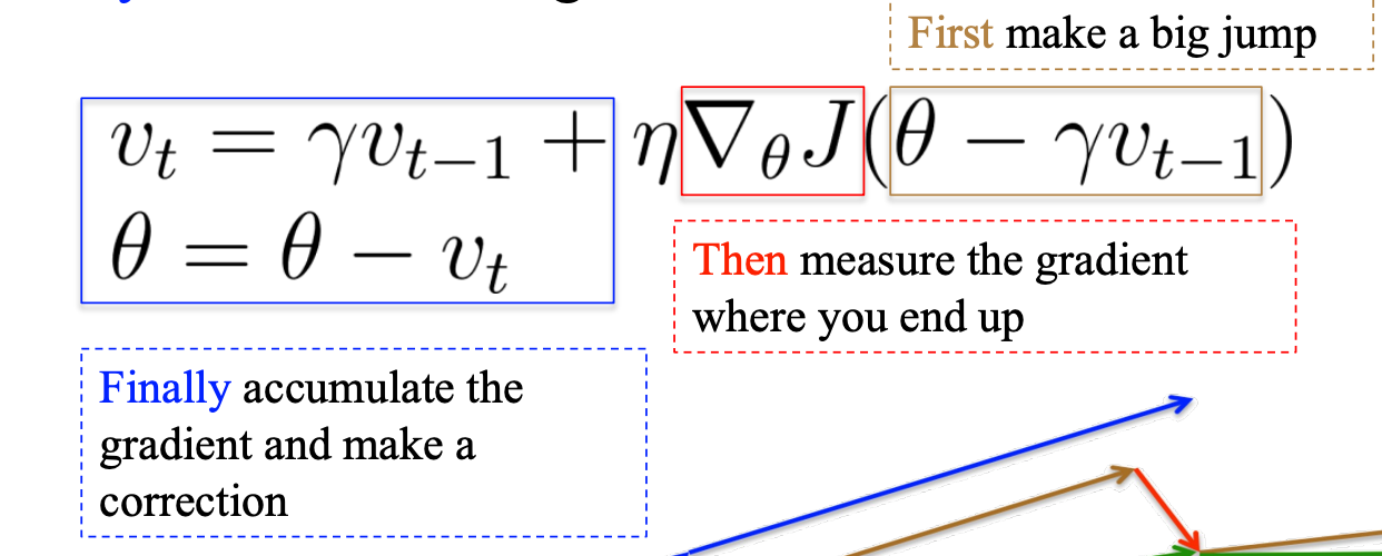
NAG:

The big jump in the standard momentum is too aggressive

So, in the Nesterov accelerated gradient use a previous gradient to big jump and a correction

theta - r v_t-1 means that update according to the previous, which is the big jump depending on the previous accumulated gradient.

Then, calculate the gradient plus the contributed previously accumulated gradient to update the theta

Adagrad:

to achieve the different learning rate for features

i means dimension

t means iteration

suitable for sparse data

but the global learning rate needed

Adadelta:

in order to deal with the problem of Adagrad(infinitesimally small for the denominator in the end), modify the gt equation as above. Contributed the last square sum of gt, and current gt.

H is the secondary gradient

with consistent units

Lecture 4 Norm

P10 weight decay

pls write the structure of the normalization

inverted, dropout-connect

BN, (reduce covariance)

R means regularisation functions, r on page 6 is the upper boundary for parameter complex

Page 24 in slide, bottom 2 are independent methods

the group right top corner is the normal training process(i.e. only train on the training set)

drop out

scale down

in the training process, each unit has with p possibility

p present

1-p disappear

in the test process, they always present

p is times the w in layer

inverted

see slide

M in slide 36 is the matrix of binary (1 or 0)

adding the extra linear function after the normalization in each layer’s output. gamma means the scale parameter, beta means the shift parameter

batch norm: norm applies in all examples in this batch in each channel

layer norm: norm applies in each data sample in this batch

instance norm: norm applies in an example in this batch in a channel

group norm: norms apply in some channels in an example (split an example into multiple parts) in a data batch

Lecture 5 CNN

P46 different sorts of pooling

Spectral pooling?

un-pooling uses the (max) location information to reverse the process, keeping the 0 at information lacking place

more previous layer, the information is more simple. (line, color block)

more higher layer, the more meaningful information included

transposed convolution is also called the deconvolution method, enlarging the feature map until keeps the same as input size

in the process of deconvolution, the output will larger, it will happen to overlap in the process, summation the overlap region. Also, it has the stride, crop (like the padding, but crop the data in the output) Output size = (N-1) S + K - 2C

In pytorch, using the sequential in init rather than init function like tut note.
the kernel in CNN is similar to the digital, tut 6 notebook

its like the mouse in 5318, get a bigger score of the kernel output

Lecture 7

dead relu means that the zero output of the relu activation function

Data augmentation is rotate, distortion, color changing etc. methods to manipulate the data.

In local response normalization, a is the center of the region

overlapping pooling, polling stride less than pooling kernel size

smaller filter means deeper, more non-linearity, fewer parameters.

p is changing to ensure the size of the output is same on the googlenet

p28, right is the google net structure, and left is the normal way. It helps to decrease the depth of the feature map in the right method.

p37 is used to avoid the overconfident of the model, with the label smoothing

1 by 1 conv layer is used to exchange the information among channels ????

Shuffle net is another way to exchange information

Extension

Ghost filter?

Lego filter?

adder filter?

Lecture 8

Lecture 9

The masked LM in BERT in used to predict the masked word by linear regression

Classification in BERT is used in the binary classifier to identify the 1 or 2 sentences

P49 the place of dot product is, output of the classifier and the representation of token, multiple numbers is because the multiple-classifier of the model, then using the result passing into the softmax to predict the final prediction

the gates in code split the matrix into multiple chunks and pass into the gates.

Lecture 10

P26: if the degree of the J is large, the information from J to I node is very small. Because the denominator is Djj Dii.

the D^-0.5 A D^-0.5(connection) H(value of each neighbour, near features) W(parameter)

Laplacian means to reduce the shape of the matrix, in the spectral matrix, the shape is quality large

Each row and each column in matrix of Laplacian are zero

the eigen matrix are used to reshape the original matrix, which similar to the PCA, focusing on the important part of the matrix

Lecture 11

the detected size of the boundary box many different. So, the resizing of the image is necessary for CNN. P16.

The proposal may overlap, it makes the duplication of calculation. P17

Fast R-CNN: instead of using the image level input like P16, the fast way is using the features in CNN as input to the bounding box task. P20

But the problem of different sizes still exists, fast R-CNN uses the max pooling way to ensure the size of the output.

Faster R-CNN: spp-net, improve at the extra pooling layer then fast R-CNN. In this model, the classification, detection, boundary box, etc tasks are all done by different CNNs.

In other words, the nature of the faster here is replacing the original image object detection by the feature object detection. It reduces the computational resources.

Mask R-CNN: deter the pixel in the image along to what label.

RoIAlign is more accurate in the pooling layer, directly dividing the result evenly without considering the number, and using the distance of each point to decide the number of the results after the max pooling.

excepted predict the xyhw, the dx,dy,dh,dw (difference of the xyhw) are also included in the prediction. Jargon called an anchor.

Lecture 12

high value in Dx, maximize the (1-D(G(z)))

Lecture 13

diffusion

GAN: 输入为随机输入

f(theta) = Y

Y 为图像

X 为随机输入

F（）为神经网络， 映射xy之间的转换关系，从正态分布到图像的分布（特殊的集合）

不用MSE的原因是 噪音和图像之前的关系没有有意义的关系，也就是梯度会没有， 并且只能生成看到过的图片， 不会生成没看见过的图片

生成式对抗模型：两个神经网络，生成式网络（生成假图）和分类器（检验真假）

生成式模型从分类起学会到如何生成真图

分类无法区分的时候，就训练完了

VAE: encoder the image, then decode it

decode之后和原始的 计算loss

从参化

diffusion: 去燥模型，退热定律

X → XT.noisy(高斯)

X → X+Theta → XT.noisy(高斯)

X → … → X+Theta * n → XT.noisy(高斯)

每次加一点点噪音， 直到纯噪音

每次加的高斯分布的噪音

loss 为检测图片中的噪音数量

反过去，就是按照噪音去预测图片

diffusion只有一个NN，其他模型为多个