Posted 2024-06-16Updated 2024-08-09USYD - Lecture

Lecture 1

N-Gram LMs

The 4 ways to deal with the unseen word sequence

smoothing:

Untitled

discounting:

Untitled

Interpolation: using the multiple N-Gram probability

Untitled

Kneser-Ney smoothing:

Lecture2

Lecture3

Lecture4

Note the formula macro and micro F1 score — ass2

Not the find_best_socre initial number should be negative — ass2

directly using average will make some features vanish (+ and -), also the order is meaningless

in slide, NER page 66

labels number * length * length means:

each token in sequence is possible for start or end, that is length * length

then, each span can be predicted as each label

so, the output should be (labels * length * length)

Untitled

Lecture 5

beam search

in nature, greedy search is to find the local optimal solution in each step

Lecture 6

the label in current word from LSTM purely, B I O possibility(sum as 1)

score = current label p * best (previous p * transfer p)

it from

score = current label p * best (i.e. DP * transfer model)

DP refers to the optimal route in choice

transfer model refers to the Markov model

co reference

dependency parsing

Lecture 7

Lecture 8

disadvantages of self-attention

problem:

non-linear lacking

order lacking

resolve:

feedforward layer

additional position vector

issue: the length of the position vector is fixed, not flexible enough
the mask is for ignoring the future word in the training process, it lets the model know what is known in this step, and what is the prediction in this step. In math, put the infinite negative value for future words and dot the product in the current word
the multiple layers of self-attention are used to build better representation of the word

query: curve line

key: embedding word

value: passing into the weighted value

Lecture 10

data can from

fineweb

common craw

Lecture 11

Review

The content below is the missing slide week.

parsing, 句法分析, identity the grammar structure by sub-phrases

The span in the sentence called the phrase

treebanks

Method: Dependency Parsing / Grammar

compute every possible dependency to find the best score

Or, choose a way to get the best overall score

co-reference

Posted 2024-06-16Updated 2024-08-09USYD - Lecture

USYD - COMP 5329

COMP 5329

Lecture 2

P9 XOR

P31 Activation

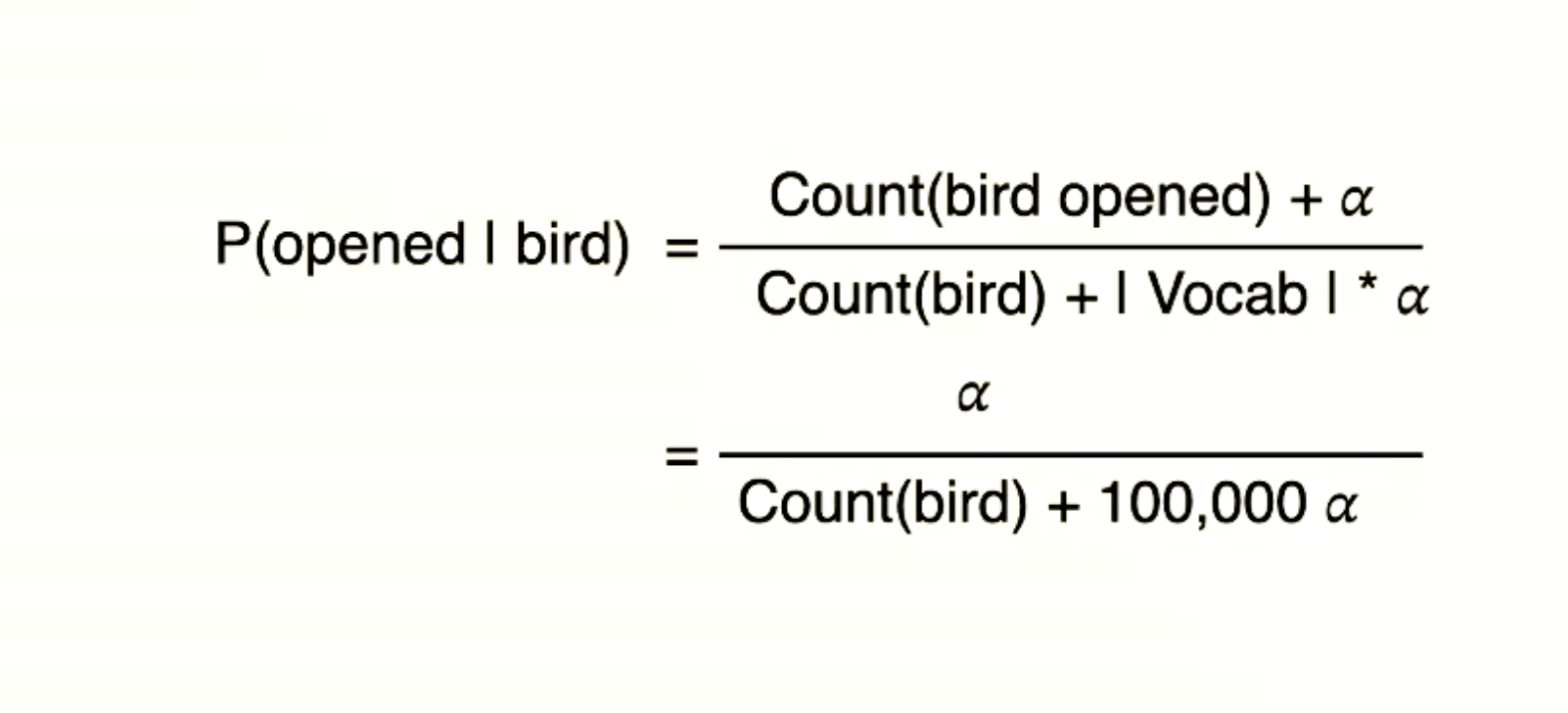
P36 CE

P37 KL, Entropy

P38 SoftMax

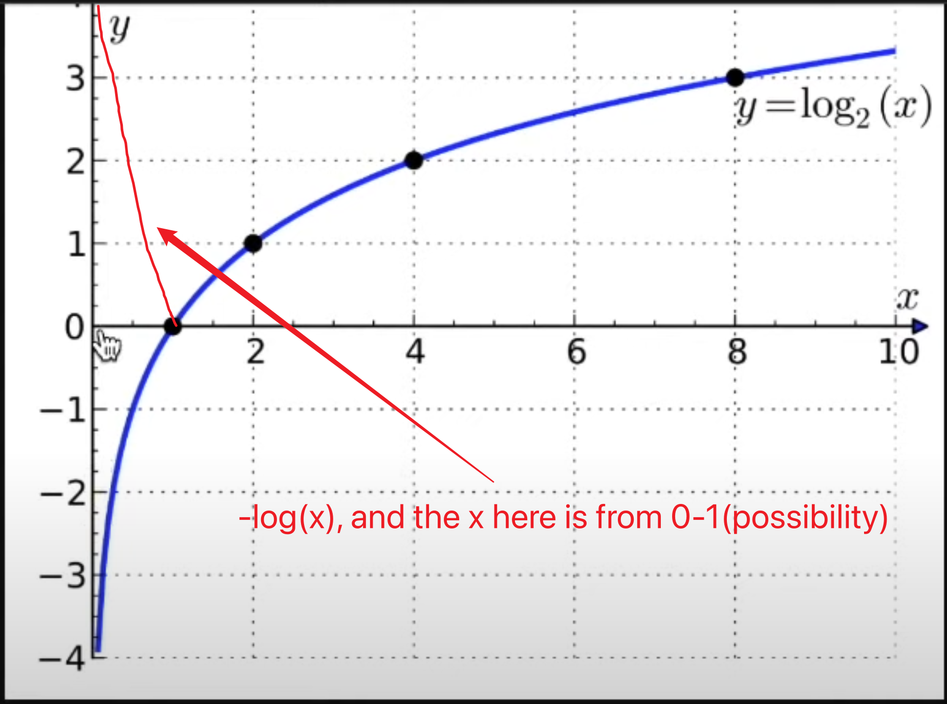
p36, p37 two attributes cross-entropy loss issue?
the disadvantage of batch gradient descent is when N is too large, the computation is very expensive, but the one example SGD only uses the single example. It may not be the best, due to the random.

mini-batches SGD: divide into mini-batches, in each epoch calculate the gradient

extension content:

sensitivity? make the back propagation similar to the feedforward

Lecture 3 GD

Different gradient descent.

Challenges: proper lr, same lr, saddle point

P9-10 Momentum

P11 NAG

P17 Adagrad

P21 Adadelta

P25 RMSprop

P26, 27 Adam

P34 Initialization

Batch Gradient descent: Accuracy

Stochastic gradient descent: efficiency

Mini-batch gradient descent: trade-off of accuracy and efficiency

Momentum is to update SGD, to accelerate and dampen oscillation

increase the momentum term in the same direction, reduce in change direction

NAG:

The big jump in the standard momentum is too aggressive

So, in the Nesterov accelerated gradient use a previous gradient to big jump and a correction

Untitled

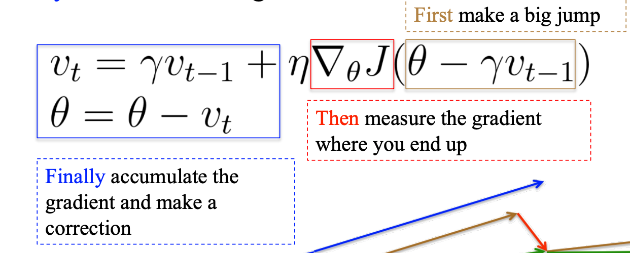
theta - r v_t-1 means that update according to the previous, which is the big jump depending on the previous accumulated gradient.

Then, calculate the gradient plus the contributed previously accumulated gradient to update the theta

Adagrad:

to achieve the different learning rate for features

i means dimension

t means iteration

suitable for sparse data

but the global learning rate needed

Adadelta:

Untitled

in order to deal with the problem of Adagrad(infinitesimally small for the denominator in the end), modify the gt equation as above. Contributed the last square sum of gt, and current gt.

H is the secondary gradient

with consistent units

Lecture 4 Norm

P10 weight decay

pls write the structure of the normalization

inverted, dropout-connect

BN, (reduce covariance)

R means regularisation functions, r on page 6 is the upper boundary for parameter complex

Page 24 in slide, bottom 2 are independent methods

the group right top corner is the normal training process(i.e. only train on the training set)

drop out

scale down

in the training process, each unit has with p possibility

p present

1-p disappear

in the test process, they always present

p is times the w in layer

inverted

see slide

M in slide 36 is the matrix of binary (1 or 0)

adding the extra linear function after the normalization in each layer’s output. gamma means the scale parameter, beta means the shift parameter

batch norm: norm applies in all examples in this batch in each channel

layer norm: norm applies in each data sample in this batch

instance norm: norm applies in an example in this batch in a channel

group norm: norms apply in some channels in an example (split an example into multiple parts) in a data batch

Lecture 5 CNN

P46 different sorts of pooling

Spectral pooling?

un-pooling uses the (max) location information to reverse the process, keeping the 0 at information lacking place

more previous layer, the information is more simple. (line, color block)

more higher layer, the more meaningful information included

transposed convolution is also called the deconvolution method, enlarging the feature map until keeps the same as input size

in the process of deconvolution, the output will larger, it will happen to overlap in the process, summation the overlap region. Also, it has the stride, crop (like the padding, but crop the data in the output) Output size = (N-1) S + K - 2C

In pytorch, using the sequential in init rather than init function like tut note.
the kernel in CNN is similar to the digital, tut 6 notebook

its like the mouse in 5318, get a bigger score of the kernel output

Lecture 7

dead relu means that the zero output of the relu activation function

Data augmentation is rotate, distortion, color changing etc. methods to manipulate the data.

In local response normalization, a is the center of the region

overlapping pooling, polling stride less than pooling kernel size

smaller filter means deeper, more non-linearity, fewer parameters.

p is changing to ensure the size of the output is same on the googlenet

p28, right is the google net structure, and left is the normal way. It helps to decrease the depth of the feature map in the right method.

p37 is used to avoid the overconfident of the model, with the label smoothing

1 by 1 conv layer is used to exchange the information among channels ????

Shuffle net is another way to exchange information

Extension

Ghost filter?

Lego filter?

adder filter?

Lecture 8

Lecture 9

The masked LM in BERT in used to predict the masked word by linear regression

Classification in BERT is used in the binary classifier to identify the 1 or 2 sentences

P49 the place of dot product is, output of the classifier and the representation of token, multiple numbers is because the multiple-classifier of the model, then using the result passing into the softmax to predict the final prediction

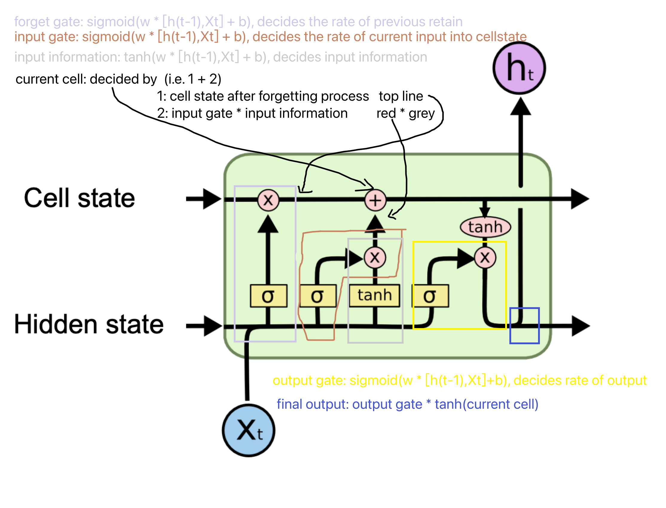
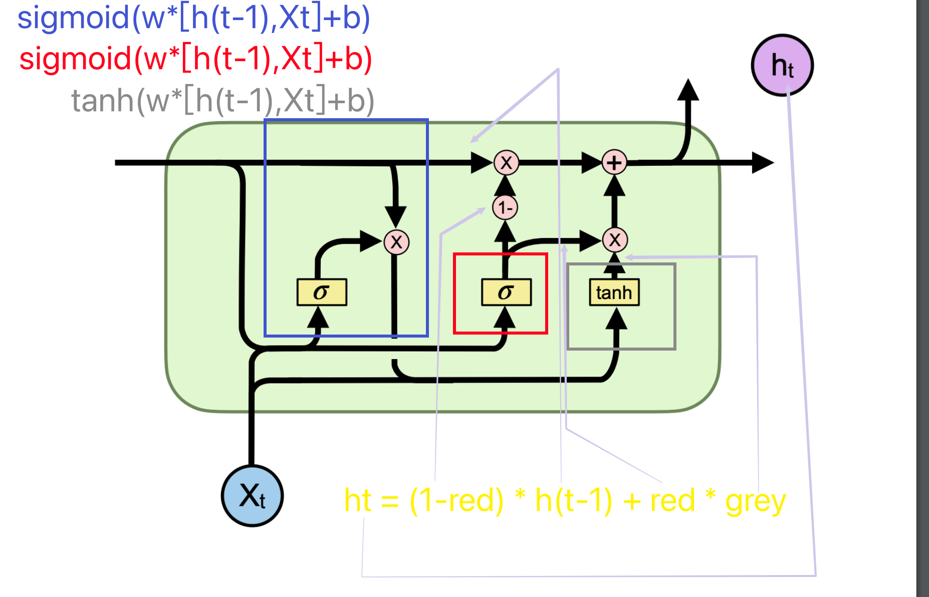
the gates in code split the matrix into multiple chunks and pass into the gates.

Lecture 10

P26: if the degree of the J is large, the information from J to I node is very small. Because the denominator is Djj Dii.

the D^-0.5 A D^-0.5(connection) H(value of each neighbour, near features) W(parameter)

Laplacian means to reduce the shape of the matrix, in the spectral matrix, the shape is quality large

Each row and each column in matrix of Laplacian are zero

Untitled

the eigen matrix are used to reshape the original matrix, which similar to the PCA, focusing on the important part of the matrix

Lecture 11

the detected size of the boundary box many different. So, the resizing of the image is necessary for CNN. P16.

The proposal may overlap, it makes the duplication of calculation. P17

Fast R-CNN: instead of using the image level input like P16, the fast way is using the features in CNN as input to the bounding box task. P20

But the problem of different sizes still exists, fast R-CNN uses the max pooling way to ensure the size of the output.

Faster R-CNN: spp-net, improve at the extra pooling layer then fast R-CNN. In this model, the classification, detection, boundary box, etc tasks are all done by different CNNs.

In other words, the nature of the faster here is replacing the original image object detection by the feature object detection. It reduces the computational resources.

Mask R-CNN: deter the pixel in the image along to what label.

RoIAlign is more accurate in the pooling layer, directly dividing the result evenly without considering the number, and using the distance of each point to decide the number of the results after the max pooling.

excepted predict the xyhw, the dx,dy,dh,dw (difference of the xyhw) are also included in the prediction. Jargon called an anchor.

Lecture 12

high value in Dx, maximize the (1-D(G(z)))

Lecture 13

diffusion

GAN: 输入为随机输入

f(theta) = Y

Y 为图像

X 为随机输入

F（）为神经网络，映射xy之间的转换关系，从正态分布到图像的分布（特殊的集合）

不用MSE的原因是噪音和图像之前的关系没有有意义的关系，也就是梯度会没有，并且只能生成看到过的图片，不会生成没看见过的图片

生成式对抗模型：两个神经网络，生成式网络（生成假图）和分类器（检验真假）

生成式模型从分类起学会到如何生成真图

分类无法区分的时候，就训练完了

VAE: encoder the image, then decode it

decode之后和原始的计算loss

从参化

diffusion: 去燥模型，退热定律

X → XT.noisy(高斯)

X → X+Theta → XT.noisy(高斯)

X → … → X+Theta * n → XT.noisy(高斯)

每次加一点点噪音，直到纯噪音

每次加的高斯分布的噪音

loss 为检测图片中的噪音数量

反过去，就是按照噪音去预测图片

diffusion只有一个NN，其他模型为多个

Posted 2024-06-16Updated 2024-06-20USYD - Lecture

USYD - DATA 5207

DATA 5207

Lecture 2

presenting data to non-expert (visualization)

less technical knowledge

making data engage

convey the pattern

Data Graphics

3 consideration

what information want to communicate

who is the target audience

why design this feature relevant

Lecture 3

confounding factors: earning by height, may it occur by gender

select the topic this weekend

RMD template

Lecture 4

better R square, better job the model does. This means the better-fitting in model

maximize the variables in the model

not only use the technic thing to fit the data but adding the theoretical thing to increase the use in practice

observational data can not make the causal inference (confounding factor included)

model error

random errors (precision limitation - sample number)

systematic error (error in research design - non-sampling error)

difference between observed and actual

response, instrument, interviewer

sample design error

selection, frame

explore dataset graphs

variables

model choice

correlation plot all variables

variable selection methods - stepwise, lasso, or

Lecture 5

limitation of the LR is assuming the relationship is linear

logits?

ordinal logistic regression (agree, very agree, etc)

For the material in lab 5, the last image can be repainted as for each year, plot the importance of each variable (independent factor) into a single panel.

Lecture 6

fuzzyjoin is a function that similar operation in SQL

Research Plan Format

Format

Hide the R chunks, the template has the code to hide

key feature should be identified

why use the LR

Literature

theory from Literature

hypothesis is for testing? is that the previous section provided

literature: tells you, communicate the hypothesis you provide

inform the things you need to do

underpin the thing you want to explain

may error in the literature section, falsify the idea

Data

api missing

operation

Limitation

can be deleted

Lecture 7 Quiz week

data can from

consumer data

social media

AB testing (to decide the better version in different versions)

for instance, the color, and size of the button may sent to users, and the amount they click to decide the better version

census

individuals include surveys

web scraping

Lecture 8

survey

system error - no random

may younger people be more likely to respond to the phone (phone survey) - nonresponse bias

The census is not like the survey, due to its not doing the data sample, according to the entire residents in the country

random error refers to sampling

Assignment-1

Economic: Q288, 50 (income)
1. 1
Occupation: Q281, 282, 283
Education: Q275
1. https://d1wqtxts1xzle7.cloudfront.net/49101438/18.01.053.20160304-libre.pdf?1474797472=&response-content-disposition=inline%3B+filename%3DEffect_of_Education_on_Quality_of_Life_a.pdf&Expires=1713509378&Signature=bTvJ~~0cklHa83ixDEhUTW02gYB4KW0iex7Mx6etlJqBNha-f0l-gvirWcVjlpbtaXdn5SsFoSsWtjeay-18z5De6i3e2wRtZvtx5cuzyJe2RLJHKYPPXrkiEORhb9c35JK~~-WjFa7T8c8OIQj5RxD11Gj3W7wCsC3jJw~~VOewTDYwkVBKXC1-7BjpWcbOSrkZnazJwulzVzLIERo0l6iO51LIqFi6wY8TSiTTdFGhiHctf9bu2Y7IapgVAwDLKXbpYTdXd3c4nVMPqQry~~YQ5iOjKVEmcCdMQwn0HUGe837Dn38-7ttCIbNASUOgpjEGQEjmNlznMsOW9jG~X9VHjw__&Key-Pair-Id=APKAJLOHF5GGSLRBV4ZA
2. https://www.sciencedirect.com/science/article/pii/S2214804314001153?via%3Dihub
Societal Wellbeing: Q47 (health)
Security: Q131-138, 52
Social capital, trust: Q57-61
1. https://link.springer.com/article/10.1007/s00148-007-0146-7 (neighbourhood only)

PCA to combine the multiple variables into one feature

Lecture 10

cable library in R

Lecture 11 - Causality

Lecture 12 - Journalism

datasplash platform

Final Project

the plots and tables can be included in the report

using the table to regression result (kable) function

Posted 2023-12-22Updated 2024-06-20Pytorch Introduction

Pytorch Tutorial 5

The reason use the NN is inner kernel of logistic regression is still linear, to avoid the linear relationship, the NN can use activation function, for instance ReLU.

In this case, we use ReLu as our activation function to predict the image, and it can be found that the accuracy is far better than LR, shows more abilities.

from os import path, mkdir
from random import randint

import torch
import numpy as np
import torchvision
from matplotlib import pyplot as plt
from torchvision.datasets import MNIST
from torchvision.transforms import ToTensor
from torch.utils.data.sampler import SubsetRandomSampler
from torch.utils.data.dataloader import DataLoader
import torch.nn.functional as F
import torch.nn as nn

dataset = MNIST(root="./data", download=True, transform=ToTensor())
test_dataset = MNIST(root='./data', train=False, transform=ToTensor())

def split_indices(n, rate):
    # create number of validation set
    n_val = int(n * rate)
    # create shuffled index from 0-n, with no repeat
    idxs = np.random.permutation(n)
    # retuen (n_val,last) index and (first n_val) index
    # i.e. training index and validation index
    return idxs[n_val:], idxs[:n_val]

train_indices, val_indices = split_indices(len(dataset), 0.2)

batch_size = 100
train_sampler = SubsetRandomSampler(train_indices)
train_loder = DataLoader(dataset,
                         batch_size,
                         sampler=train_sampler)

val_sampler = SubsetRandomSampler(val_indices)
val_loder = DataLoader(dataset,
                       batch_size,
                       sampler=val_sampler)

input_size = 28 * 28
num_classes = 10

class MnistModel(nn.Module):

    def __init__(self, in_size, hidden_size, out_size):
        super().__init__()

        self.linear1 = nn.Linear(in_size, hidden_size)

        self.linear2 = nn.Linear(hidden_size, out_size)

    def forward(self, xb):
        # flatten
        xb = xb.view(xb.size(0), -1)
        # xb = xb.reshape(xb.size(0), -1)
        return self.linear2(F.relu(self.linear1(xb)))

# for t in model.parameters():
#     print(t.shape)

# for img, labels in train_loder:
#     outputs = model(img)
#     loss = F.cross_entropy(outputs, labels)
#     break

def get_device():
    if torch.cuda.is_available():
        return torch.device('cuda')
    else:
        return torch.device('cpu')

def to_device(data, device):
    if isinstance(data, (list, tuple)):
        return [to_device(x, device) for x in data]
    return data.to(device, non_blocking=True)

# for img, label in train_loder:
#     print(img.shape)
#     img = to_device(img, device)
#     print(img.device)
#     break

class DeviceDataLoder():
    def __init__(self, dl, device):
        self.dl = dl
        self.device = device

    def __iter__(self):
        # lazy load here
        # instead of load data into device each time, instead, load each batch
        for b in self.dl:
            yield to_device(b, self.device)

    def __len__(self):
        return len(self.dl)

# use DeviceDataLoader as warpper
train_dl = DeviceDataLoder(train_loder, get_device())
valid_dl = DeviceDataLoder(val_loder, get_device())

def loss_batch(model, loss_func, xb, yb, opt=None, metric=None):
    preds = model(xb)

    loss = loss_func(preds, yb)

    if opt is not None:
        loss.backward()
        opt.step()
        opt.zero_grad()

    metric_result = None
    if metric is not None:
        metric_result = metric(preds, yb)

    return loss.item(), len(xb), metric_result

def evaluate(model, loss_func, valid_dl, metric=None):
    with torch.no_grad():
        results = [loss_batch(model, loss_func, xb, yb, metric=metric)
                   for xb, yb in valid_dl]

        # separate the lists
        loss, nums, metric = zip(*results)
        total = np.sum(nums)
        avg_loss = np.sum(np.multiply(loss, nums)) / total
        avg_metric = None
        if metric is not None:
            avg_metric = np.sum(np.multiply(metric, nums)) / total
    return avg_loss, total, avg_metric

def fit(epochs, lr, model, loss_func, train_dl, valid_dl, opt_fn=None, metric=None):
    if opt_fn is None:
        opt_fn = torch.optim.SGD
    opt = opt_fn(model.parameters(), lr=lr)
    loss_history = []
    metric_history = []

    for epoch in range(epochs):
        for xb, yb in train_dl:
            loss_batch(model, loss_func, xb, yb, opt)
        result = evaluate(model, loss_func, valid_dl, metric)
        val_loss, total, val_metric = result

        loss_history.append(val_loss)
        metric_history.append(val_metric)

        if metric is not None:
            print(f'Epoch [{epoch + 1}/{epochs}], Loss: {val_loss:.4f}, Metric: {val_metric:.4f}')
        else:
            print(f'Epoch [{epoch + 1}/{epochs}], Loss: {val_loss:.4f}')

    return loss_history, metric_history

def accuracy(output, label):
    _, preds = torch.max(output, dim=1)
    return torch.sum(label == preds).item() / len(preds)

model = MnistModel(input_size, 32, num_classes)
to_device(model, get_device())

if path.exists('./tutorial5/mnist-logistic.pth'):
    model.load_state_dict(torch.load('./tutorial5/mnist-logistic.pth'))

else:
    loss_history, metric_history = fit(5, 0.5, model, F.cross_entropy,
                                       train_dl,
                                       valid_dl,
                                       opt_fn=torch.optim.SGD,
                                       metric=accuracy)
    # it will save the weight and bias for this model
    # new dir
    mkdir('./tutorial5')
    torch.save(model.state_dict(), './tutorial5/mnist-logistic.pth')

def prediction_img(img, model):
    xb = img.unsqueeze(0)
    yb = model(xb)
    _, preds = torch.max(yb, dim=1)
    return preds[0].item()

for i in range(10):
    img, label = test_dataset[randint(0, len(test_dataset) - 1)]
    img_np = np.array(img)
    plt.imshow(img_np.squeeze(), cmap='gray')
    plt.show()
    print(prediction_img(img, model))

Posted 2023-12-22Updated 2024-06-20Pytorch Introduction

Pytorch Tutorial 3

simple linear regression with bulit in tools in pytorch

generate prediction
calculate the loss
compute gradients of w and b
adjust w and b
reset gradients to zero

these 5 steps also respect to the loop in the next function

import numpy as np
import torch.nn as nn
import torch
from torch.utils.data import TensorDataset
from torch.utils.data import DataLoader
import torch.nn.functional as F

# temp, rainfall, humidity
# inputs = torch.tensor(np.random.uniform(0, 120, size=(15, 3)))
# the input and output here need to specify the dtype, otherwise, when torch generate the prediction,
# it will encounter the problem of dtype is not match
inputs = torch.tensor(np.array(
    [[109.4144, 11.2775, 32.4521], [2.0002, 47.0248, 49.9469], [27.1528, 57.8907, 91.2076],
     [44.8227, 71.6239, 64.0752], [66.0968, 92.5966, 94.0775], [59.6257, 76.9701, 92.1656],
     [8.1551, 1.7426, 10.5297], [112.6036, 47.2793, 95.4221], [3.2212, 61.8274, 115.9187],
     [35.0351, 110.6133, 66.6992], [8.8387, 21.8008, 50.0480], [68.7698, 59.9815, 12.0230],
     [111.3881, 90.3050, 62.1327], [101.7462, 115.7447, 33.4925], [27.7659, 54.5803, 105.3599]], dtype='float32'))

# apples, oranges
# targets = torch.tensor(np.random.uniform(0, 50, size=(15, 2)))
targets = torch.tensor(np.array(
    [[28.1090, 45.0061], [29.0839, 6.4205], [35.2633, 44.1196],
     [29.5371, 6.8457], [7.4298, 36.1434], [6.6296, 47.1809],
     [49.9750, 49.9321], [34.1796, 16.6732], [46.8875, 7.6084],
     [23.0442, 42.2229], [29.7401, 13.4199], [3.0854, 21.4550],
     [47.6801, 49.1518], [18.7320, 18.4418], [34.2725, 25.8721]], dtype='float32'))
# print(inputs)
# print(targets)

# TensorDataset will creat the structure of pairing (input and target) accordingly
train_ds = TensorDataset(inputs, targets)

batch_size = 5
train_dl = DataLoader(train_ds, batch_size, shuffle=True)

# Each batch size is 5, and the data are shuffled
# and is still can contain the pair of data, the structure won't be shuffled
# for xb, yb in train_dl:
#     print("batch:")
#     print(xb)
#     print(yb)

# specify the input and output feature number
model = nn.Linear(3, 2)
# the weight and bias will be initialed automatically, and the parameter of requires_grad will be set as True
# print(model.weight)
# print(model.bias)
# print(list(model.parameters()))

# preds = model(inputs)
# print(preds)

loss_fn = F.mse_loss
loss = loss_fn(model(inputs), targets)
# print(loss)

opt = torch.optim.SGD(model.parameters(), lr=1e-5)

# 1 generate prediction
# 2 calculate the loss
# 3 compute gradients of w and b
# 4 adjust w and b
# 5 reset gradients to zero
# these 5 steps also respect to the loop in the next function

def fit(num_epochs, model, loss_fn, opt):
    # training interation
    for epoch in range(num_epochs):
        # batches in each interation
        for xb, yb in train_dl:
            pred = model(xb)
            loss = loss_fn(pred, yb)
            loss.backward()
            opt.step()
            opt.zero_grad()
        if (epoch+1) % 10 == 0:
            print('Epoch [{}/{}], Loss: {:.4f}'.format(epoch+1, num_epochs, loss.item()))

fit(100, model, loss_fn, opt)

Posted 2023-12-21Updated 2024-08-09Pytorch Introduction

Pytorch Tutorial 4

load dataset
1. transform the data into tensor
split the dataset into training, testing, validation datasets
1. define the function of indices shuffle (the dataset are ordered, if missing apply the shuffle, the individual dataset may only contains one label)
2. create sampler and loader
customise the MnistModel function
define loss_batch
1. calculate loss in current batch
define evaluate
1. calculate average loss in batches
define accuracy
1. also called metric to shows the accuracy
create fit function
1. epoch loop
  1. train loop
    1. loss_batch — for train
  2. evaluate result
  3. print result
call fit

from os import path
from random import randint

import torch
import torchvision
from torchvision.datasets import MNIST
import matplotlib.pyplot as plt
import numpy as np
from torch.utils.data.dataloader import DataLoader
from torch.utils.data.sampler import SubsetRandomSampler
import torch.nn as nn
import torch.nn.functional as F

# transoforms used to transform the MNIST dataset into tensor in order to torch can work with
import torchvision.transforms as transforms

# here the datasets in original format, can not be understood by torch
datasets = MNIST(root='./data', download=True)
# print(len(datasets))

test_dataset = MNIST(root='./data', train=False, transform=transforms.ToTensor())
# print(len(test_dataset))

# img, label = datasets[0]
# plt.imshow(img, cmap='gray')
# plt.show()

# print(label)

# here the dataset is already transformed into tensor
dataset = MNIST(root='./data', download=True, transform=transforms.ToTensor())

# the shape here is 1,28,28, color, height, weight
# img_tensor, label = dataset[0]
# print(img_tensor.shape, label)

# print(img_tensor[:, 10:15, 10:15])
# print(torch.max(img_tensor), torch.min(img_tensor))
# plt.imshow(img_tensor[0, 10:15, 10:15], cmap='gray')
# plt.show()

def split_indices(n, rate):
    # create number of validation set
    n_val = int(n * rate)
    # create shuffled index from 0-n, with no repeat
    idxs = np.random.permutation(n)
    # retuen (n_val,last) index and (first n_val) index
    # i.e. training index and validation index
    return idxs[n_val:], idxs[:n_val]

train_indices, val_indices = split_indices(len(dataset), 0.2)
# print(len(train_indices), len(val_indices))

# the sampler here is randomly select the indices from list with number of batch_size
# the reason for this is lower down the training time and computation
# and utilize multiple epoch to train the model, if not, the training will deal with whole data set,
# that will occupy too much memory space and make too much pressure to computational resources.
# in this case, the training process will transfer to smaller chucks
batch_size = 100
train_sampler = SubsetRandomSampler(train_indices)
train_loder = DataLoader(dataset,
                         batch_size,
                         sampler=train_sampler)

val_sampler = SubsetRandomSampler(val_indices)
val_loder = DataLoader(dataset,
                       batch_size,
                       sampler=val_sampler)

input_size = 28 * 28
num_classes = 10

# model = nn.Linear(input_size, num_classes)

# print(model.weight.shape)
# print(model.bias.shape)
#
# print(model.weight)
# print(model.bias)

# for img, label in train_loder:
#     print(img.shape)
#     print(label)
#     # there is a error, the shape of image is 1*28*28, but the received input shape was set 784
#     # so, the customized model are needed.
#     print(model(img))
#     break

class MnistModel(nn.Module):
    def __init__(self):
        super().__init__()
        # define the input and output for linear
        self.linear = nn.Linear(input_size, num_classes)

    def forward(self, xb):
        # reshape -1 here avoid the hard code, it will calculate the first dimension number
        xb = xb.reshape(-1, input_size)
        # pass the batch data to linear layer
        out = self.linear(xb)
        return out

model = MnistModel()

# the weight and bias are in the linear(model.linear.weight), instead of the model above(model.weight)
# print(model.linear.weight.shape)
# print(model.linear.bias.shape)
#
# print(model.linear.weight)
# print(model.linear.bias)

def accuracy(l1, l2):
    return torch.sum(l1 == l2).item() / len(l2)

Log plot presentation

Untitled

# for img, label in train_loder:
# the img pass in the model shape is 100,1,28,28
# the output shape is 100,10
# which reaches what we expected (represent the 0-9 digital number)
# here the softmax can be introduced to show the possibility with each number correspondingly
# possibility = e^y_i / sum(e^y_i)
# outputs = model(img)
# the second parameter here indicates the dim index need to be applied
# so 0 means the column direction, and 1 for row direction for 2D matrix
# probs = F.softmax(outputs, 1)
# print(probs.shape)
# so now the probs shape is 100,10, but each value each row represent possibility(0-1), and sum of each row is 1
# print(outputs.shape)
# print(outputs[0])
# max_probs, predicted_labels = torch.max(probs, 1)
# print(accuracy(predicted_labels, label))

# now, we need to define the loss function
# here the cross entropy is most suitable for logistic regression
# i.e.
# the true label 9 is represented vector of [0,0,0,0,0,0,0,0,0,1]
# the predict vector [0.1,0.2,0.3,0.4,0.5,0.6,0.7,0.8,0.9] for instance
# and the cross entropy is -ln(y*y_pred) i.e. -ln(1*0.9) = 0.10, which is low

# but, when the prediction is poor
# the true label 1 is represented vector of [0,1,0,0,0,0,0,0,0,0]
# the predict vector [0.1,0.2,0.3,0.4,0.5,0.6,0.7,0.8,0.9] for instance
# and the cross entropy is -ln(y*y_pred) i.e. -ln(1*0.2) = 1.6, which is high

# in the cross entropy, we only consider the right label, and ignore the other, because their vector is 0

# so when low possibility for the correct number the cross entropy(loss) is high, v.v

# define the loss function for current batch
# loss = F.cross_entropy(outputs, label)

# the equation here is -e.pow(right prediction possibility)=loss
# so the right possibility is e.pow(-loss)
# learn_rate = 0.001
# optimizer = torch.optim.SGD(model.parameters(), lr=learn_rate)
# optimizer.step()
# break

def loss_batch(model, loss_func, xb, yb, opt=None, metric=None):
    preds = model(xb)
    loss = loss_func(preds, yb)

    if opt is not None:
        loss.backward()
        opt.step()
        opt.zero_grad()

    # metric is used for model evaluation
    metric_result = None
    if metric is not None:
        metric_result = metric(preds, yb)

    return loss.item(), len(xb), metric_result

def evaluate(model, loss_func, valid_dl, metric=None):
    with torch.no_grad():
        results = [loss_batch(model, loss_func, xb, yb, metric=metric)
                   for xb, yb in valid_dl]

        # separate the lists
        loss, nums, metric = zip(*results)
        total = np.sum(nums)
        avg_loss = np.sum(np.multiply(loss, nums)) / total
        avg_metric = None
        if metric is not None:
            avg_metric = np.sum(np.multiply(metric, nums)) / total
    return avg_loss, total, avg_metric

def accuracy(output, label):
    _, preds = torch.max(output, dim=1)
    return torch.sum(label == preds).item() / len(preds)

# avg_loss, total, val_acc = evaluate(model, F.cross_entropy, val_loder, metric=accuracy)
# print("Loss: {:.4f}, total:{:.4f}, Accuracy: {:.4f}".format(avg_loss, total, val_acc))

def fit(epochs, model, loss_fn, opt, train_dl, valid_dl, metric=None):
    for epoch in range(epochs):
        for xb, yb in train_dl:
            loss, _, _ = loss_batch(model, loss_fn, xb, yb, opt, metric=metric)

        result = evaluate(model, loss_fn, valid_dl, metric=metric)
        val_loss, total, val_metric = result

        if metric is None:
            print("Epoch [{}/{}], total:{:.4f}, Loss: {:.4f}"
                  .format(epoch + 1, epochs, total, val_loss, val_metric))
        else:
            print("Epoch [{}/{}], total:{:.4f}, Loss: {:.4f}, {}: {:.4f}"
                  .format(epoch + 1, epochs, total, val_loss, metric.__name__, val_metric))

model = MnistModel()

# if path is not blank
if path.exists('mnist-logistic.pth'):
    model.load_state_dict(torch.load('mnist-logistic.pth'))

else:
    fit(5,
        model,
        F.cross_entropy,
        torch.optim.SGD(model.parameters(), lr=0.001),
        train_loder,
        val_loder,
        metric=accuracy)
    # it will save the weight and bias for this model
    torch.save(model.state_dict(), 'mnist-logistic.pth')

# read the saved model into instance
# model2 = MnistModel()
# model2.load_state_dict(torch.load('mnist-logistic.pth'))
# model2.state_dict()

def prediction_img(img, model):
    xb = img.unsqueeze(0)
    yb = model(xb)
    _, preds = torch.max(yb, dim=1)
    return preds[0].item()

for i in range(10):
    img, label = test_dataset[randint(0, len(test_dataset) - 1)]
    img_np = np.array(img)
    plt.imshow(img_np.squeeze(), cmap='gray')
    plt.show()
    print(prediction_img(img, model))

Question

when import test_dataset missing the parameter of transform, made the validation section encounter the problem of img no squeeze parameter
zip(*results), used for unpack the tuples, and pass into multiple instances
avg_loss = np.sum(np.multiply(loss, nums)) / total the reason use multiply here is for last batch number, is might not equals to previous number

Posted 2023-12-20Updated 2024-06-20Pytorch Introduction

Pytorch Tutorial 1

import torch
import numpy as np

t1 = torch.tensor(4.)
print(t1)
print(t1.dtype)

t2 = torch.tensor([1., 2, 3, 4])
print(t2)
print(t2.dtype)
# in this case the all data will be transformed to same data type
# [1., 2., 3., 4.]

t3 = torch.tensor([1., 2, 3, 4])
print(t3)
print(t3.dtype)

t4 = torch.tensor([[1, 2], [1., 4], [4, 3], [5, 6]])
print(t4)
print(t4.dtype)

print(t1.shape)
print(t2.shape)
print(t3.shape)
print(t4.shape)

# ---
x = torch.tensor(3., requires_grad=True)
w = torch.tensor(4., requires_grad=True)
b = torch.tensor(5., requires_grad=True)

y = w * x + b
print(y)
y.backward()

print(x.grad)
print(w.grad)
print(b.grad)

#  convert numpy to torch
x = np.array([[1, 2], [2, 4]])

# use shared memory space, not copy
y = torch.from_numpy(x)

#  copy data
y = torch.tensor(x)

print(y)
print(y.dtype)

# convert torch to numpy
z = y.numpy()
print(z)

Posted 2023-12-20Updated 2024-06-20Pytorch Introduction

Pytorch Tutorial 2

simple linear regression with auto gradient method in pytorch

@ means inner dot
.t() means transpose matrix
.numel() means number of element in matrix
with torch.no_grad() means code insider this block will not track gradients to save memory and computation time

import torch
import numpy as np

inputs = np.array([[0, 0, 3],
                   [0, 1, 9],
                   [1, 0, 8],
                   [1, 1, 28]], dtype='float32')

outputs = np.array([[0, 1],
                    [9, 4],
                    [7, 3],
                    [6, 7]], dtype='float32')

inputs = torch.from_numpy(inputs)
outputs = torch.from_numpy(outputs)

w = torch.randn(2, 3, requires_grad=True)
b = torch.randn(2, requires_grad=True)

# print(b)

def model(x):
    # the b is the vector, when the matrix plus b, the b will be copy bunch of data to make it as the matrix
    return x @ w.t() + b

def mse(t1, t2):
    return torch.sum((t1 - t2) ** 2) / t1.numel()

learning_rate = 1e-5
for t in range(500):
    y_pred = model(inputs)
    loss = mse(y_pred, outputs)
    loss.backward()
    with torch.no_grad():
        w -= learning_rate * w.grad
        b -= learning_rate * b.grad
        w.grad.zero_()
        b.grad.zero_()
    print(loss.item())

Lecture 1

Lecture2

Lecture3

Lecture4

Lecture 5

Lecture 6

Lecture 7

Lecture 8

Lecture 10

Lecture 11

Review

COMP 5329

Lecture 2

Lecture 3 GD

Different gradient descent.

Lecture 4 Norm

Lecture 5 CNN

Lecture 7

Lecture 8

Lecture 9

Lecture 10

Lecture 11

Lecture 12

Lecture 13

DATA 5207

Lecture 2

Lecture 3

Lecture 4

Lecture 5

Lecture 6

Research Plan Format

Format

Literature

Data

Limitation

Lecture 7 Quiz week

Lecture 8

Assignment-1

Lecture 10

Lecture 11 - Causality

Lecture 12 - Journalism

Final Project

Question

Categories

Recents

Archives

Tags